오픈소스(R) 프로그래밍 2
데이터 탐색하기

이상일(서울대학교 지리교육과 교수)

2026-01-01

기본 개념

데이터사이언스 프로세스

https://r4ds.hadley.nz/whole-game.html

탐색적 데이터 분석: 개념

• 탐색적 데이터 분석은 데이터와의 끝임없는 상호작용을 통해 의미있는 결과물을 얻어내는 과정을 의미한다. 데이터사이언스가 데이터로부터 이해, 지식, 통찰력을 획득하는 과정이라고 했을 때, 탐색적 데이터 분석은 데이터사이언스의 심장이라 해도 과언이 아니다. 상호작용은 데이터와의 질의응답의 연쇄과정을 의미한다. 의미있는 질문에 답을 얻기 위해서는 거의 반드시 데이터를 변형하거나 시각화해야만 한다.
• 데이터 변형과 데이터 시각화는 개별적으로 탐색적 데이터 분석에 기여한다. 데이터 변형은 데이터를 다른 각도로 바라볼 수 있게 해주고 다양한 요약 통계값을 산출해 준다. 데이터 시각화는 데이터에 차원을 부가함으로써 시각화 되지 않았다면 발견할 수 없었던 것을 발견할 수 있게 해준다.

탐색적 데이터 분석: 개념

• 데이터 변형에서 데이터 시각화로 이어지는 시퀀스가 탐색적 데이터 분석의 핵심적인 방법론이다. 데이터 변형의 궁극적인 목적은 바로 데이터 시각화를 위한 준비이다. 특정한 형태의 시각화를 위해서는 특정한 형태로 변형된 데이터가 필수적이고, 그러한 과정이 이해, 지식, 통찰력의 획득으로 나아가게 해주는 주된 경로이다.

• 데이터 시각화의 두 가지 목적은 탐색과 커뮤니케이션이다. 우리가 데이터 시각화를 하는 첫번째 목적은 데이터에 대한 질문에 답을 찾기 위해서이다. 우리가 데이터를 시각화하는 두 번째 목적은 우리가 발견한 것을 다른 사람들과 ‘잘’ 커뮤니케이션하기 위해서이다.

탐색적 데이터 분석: 개념

• 의미있는 질문을 생성한다.

• 질문에 답할 수 있는 그래픽(플롯, 지도 등)을 구상한다.

• 구상한 그래픽에 부합하도록 데이터를 변형한다.

• 변형한 데이터를 구상한 그래픽으로 시각화한다.

• 그래픽으로부터 질문의 답을 구하고, 더 나아가 지식, 이해, 통찰을 이끌어 낸다.

세 가지 예제

예제 데이터: gapminder

• Gapminder 재단

• R의 gapminder 패키지

• 기간: 1952-2007년 5년 단위(12개 시점)

• 국가 수: 142개국

• 관측치 수: 1,704개 (142 x 12)

• 변수: country(국가명), continent(대륙), year(연도), lifeExp(기대수명), pop(인구 수), gdpPercap(1인당 GDP)

• 동영상: https://www.youtube.com/watch?v=GmEKpKEakmQ

예제 데이터: gapminder

library(tidyverse)
library(gapminder)
gapminder

# A tibble: 1,704 × 6
   country     continent  year lifeExp      pop gdpPercap
   <fct>       <fct>     <int>   <dbl>    <int>     <dbl>
 1 Afghanistan Asia       1952    28.8  8425333      779.
 2 Afghanistan Asia       1957    30.3  9240934      821.
 3 Afghanistan Asia       1962    32.0 10267083      853.
 4 Afghanistan Asia       1967    34.0 11537966      836.
 5 Afghanistan Asia       1972    36.1 13079460      740.
 6 Afghanistan Asia       1977    38.4 14880372      786.
 7 Afghanistan Asia       1982    39.9 12881816      978.
 8 Afghanistan Asia       1987    40.8 13867957      852.
 9 Afghanistan Asia       1992    41.7 16317921      649.
10 Afghanistan Asia       1997    41.8 22227415      635.
# ℹ 1,694 more rows

질문 1

아시아의 1957년과 2007년의 1인당 GDP는 얼마이며 순위는 어떠한가? 1인당 GDP의 순위가 상승하였는가?

질문 1

• 데이터
• 결과
• 코드

# A tibble: 1,704 × 6
   country     continent  year lifeExp      pop gdpPercap
   <fct>       <fct>     <int>   <dbl>    <int>     <dbl>
 1 Afghanistan Asia       1952    28.8  8425333      779.
 2 Afghanistan Asia       1957    30.3  9240934      821.
 3 Afghanistan Asia       1962    32.0 10267083      853.
 4 Afghanistan Asia       1967    34.0 11537966      836.
 5 Afghanistan Asia       1972    36.1 13079460      740.
 6 Afghanistan Asia       1977    38.4 14880372      786.
 7 Afghanistan Asia       1982    39.9 12881816      978.
 8 Afghanistan Asia       1987    40.8 13867957      852.
 9 Afghanistan Asia       1992    41.7 16317921      649.
10 Afghanistan Asia       1997    41.8 22227415      635.
# ℹ 1,694 more rows

# A tibble: 10 × 5
# Groups:   year [2]
    year continent    sum_pop sum_gdp gdp_percap_cont
   <int> <fct>          <dbl>   <dbl>           <dbl>
 1  1957 Oceania     11941976 1.34e11          11192.
 2  1957 Americas   386953916 3.52e12           9098.
 3  1957 Europe     437890351 3.30e12           7535.
 4  1957 Africa     264837738 3.83e11           1445.
 5  1957 Asia      1562780599 1.56e12            998.
 6  2007 Oceania     24549947 8.07e11          32885.
 7  2007 Europe     586098529 1.48e13          25244.
 8  2007 Americas   898871184 1.94e13          21603.
 9  2007 Asia      3811953827 2.07e13           5432.
10  2007 Africa     929539692 2.38e12           2561.

gapminder |> 
  group_by(year, continent) |> 
  summarize(
    sum_pop = sum(pop),
    sum_gdp = sum(pop * gdpPercap),
    gdp_percap_cont = sum_gdp / sum_pop
  ) |> 
  filter(year %in% c(1957, 2007)) |> 
  arrange(year, desc(gdp_percap_cont))

질문 2

대륙별 최대국(인구가 가장 많은 나라)이 소속 대륙 전체에서 차지하는 비중이 어느 정도이고 대륙별로 어느 정도의 차이가 있는지, 그리고 대륙별 최대국의 비중이 시간이 지남에 따라 어떠한 변화 양상을 보여주고 있고, 그러한 양상에 대륙별 차이가 있는지의 여부

질문 2

• 데이터
• 그래프 1
• 코드 1
• 코드 2
• 그래프 2

# A tibble: 1,704 × 6
   country     continent  year lifeExp      pop gdpPercap
   <fct>       <fct>     <int>   <dbl>    <int>     <dbl>
 1 Afghanistan Asia       1952    28.8  8425333      779.
 2 Afghanistan Asia       1957    30.3  9240934      821.
 3 Afghanistan Asia       1962    32.0 10267083      853.
 4 Afghanistan Asia       1967    34.0 11537966      836.
 5 Afghanistan Asia       1972    36.1 13079460      740.
 6 Afghanistan Asia       1977    38.4 14880372      786.
 7 Afghanistan Asia       1982    39.9 12881816      978.
 8 Afghanistan Asia       1987    40.8 13867957      852.
 9 Afghanistan Asia       1992    41.7 16317921      649.
10 Afghanistan Asia       1997    41.8 22227415      635.
# ℹ 1,694 more rows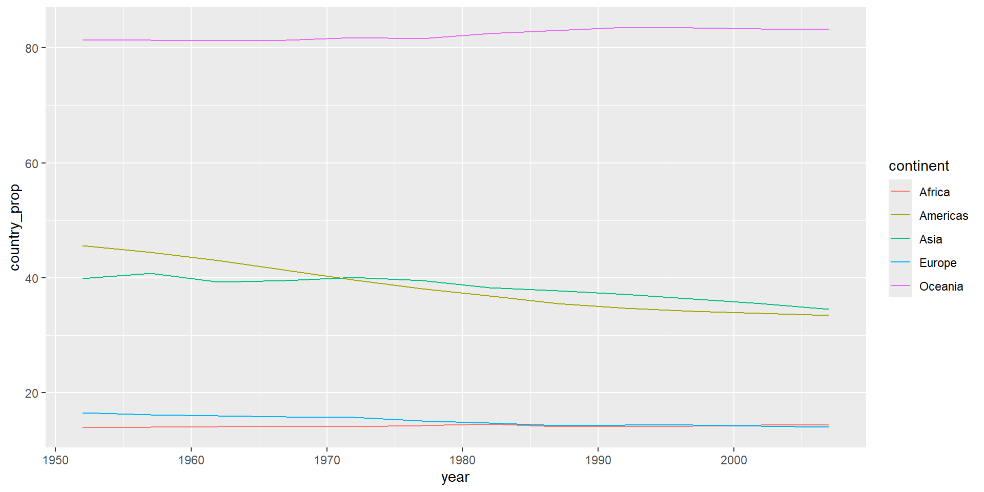

gapminder |> 
  group_by(year, continent) |> 
  mutate(
    sum_cont = sum(pop),
    country_prop = pop * 100 / sum_cont
  ) |> 
  slice_max(country_prop) |> 
  ggplot() +
  geom_line(aes(x = year, y = country_prop, color = continent))

gapminder |> 
  group_by(year, continent) |> 
  mutate(
    sum_cont = sum(pop),
    country_prop = pop * 100 / sum_cont
  ) |> 
  slice_max(country_prop) |> 
  ggplot() +
  geom_line(aes(x = year, y = country_prop, color = continent), linewidth = 1) +
  scale_x_continuous(breaks = seq(1952, 2007, 5)) +
  labs(x = "Year", y = "% of Population", color = "Continents")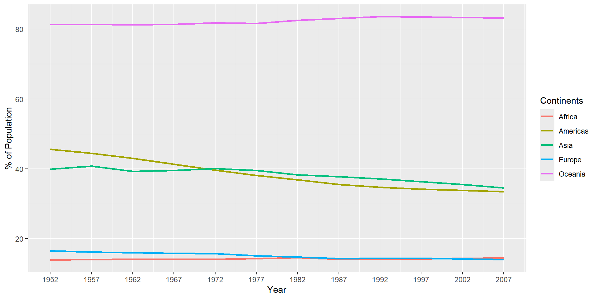

질문 3

1952~2007년간의 연평균 인구성장률의 대륙간 차이와 대륙 내 국가간 편차를 동시에 탐색

• 연평균 인구성장률(%)은 다음의 공식에 의거해 산출

\[ r=\frac{1}{n}\times\ln(\frac{P_n}{P_0})\times100 \]

질문 3

• 데이터
• 그래프 1
• 코드 1
• 코드 2
• 그래프 2

# A tibble: 1,704 × 6
   country     continent  year lifeExp      pop gdpPercap
   <fct>       <fct>     <int>   <dbl>    <int>     <dbl>
 1 Afghanistan Asia       1952    28.8  8425333      779.
 2 Afghanistan Asia       1957    30.3  9240934      821.
 3 Afghanistan Asia       1962    32.0 10267083      853.
 4 Afghanistan Asia       1967    34.0 11537966      836.
 5 Afghanistan Asia       1972    36.1 13079460      740.
 6 Afghanistan Asia       1977    38.4 14880372      786.
 7 Afghanistan Asia       1982    39.9 12881816      978.
 8 Afghanistan Asia       1987    40.8 13867957      852.
 9 Afghanistan Asia       1992    41.7 16317921      649.
10 Afghanistan Asia       1997    41.8 22227415      635.
# ℹ 1,694 more rows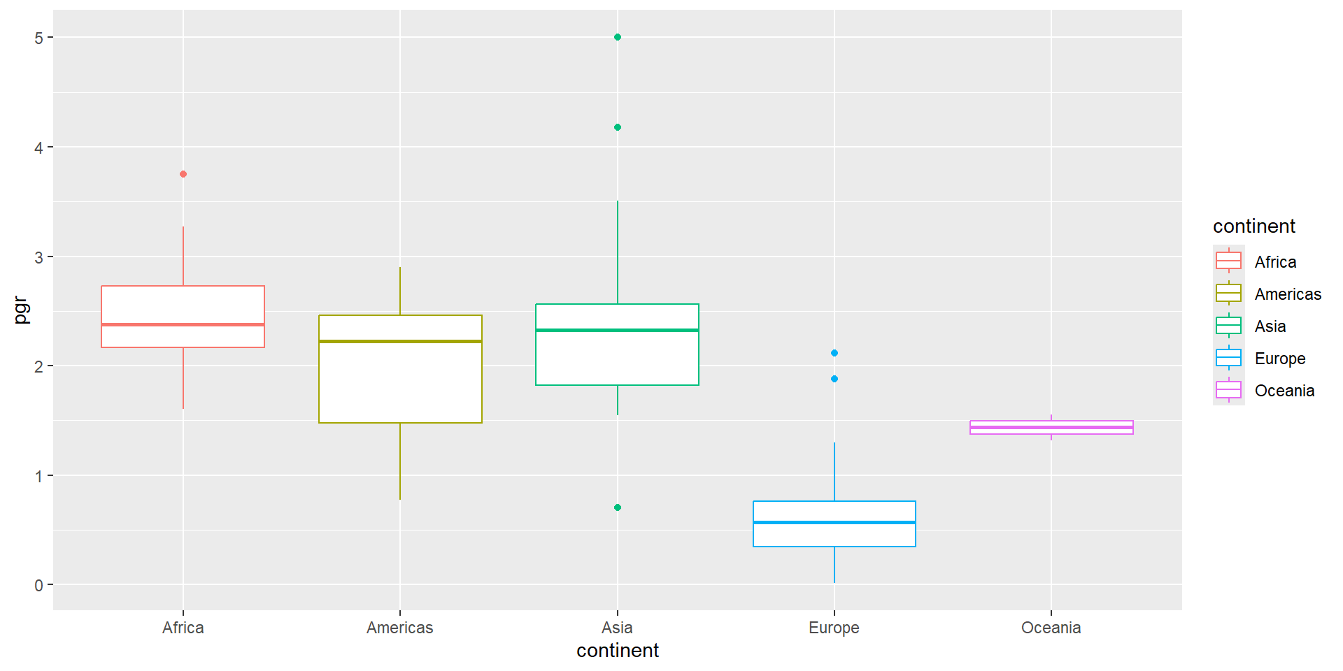

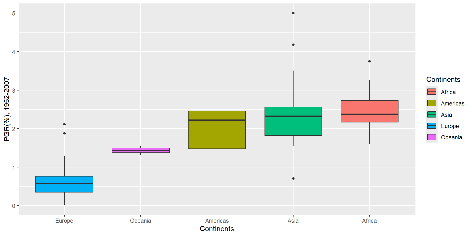
gapminder |> 
  pivot_wider(
    id_cols = c(country, continent),
    names_from = year,
    values_from = pop
  ) |> 
  mutate(
    pgr = (1/(2007-1952))*log(`2007`/`1952`) * 100
  ) |> 
  ggplot(aes(x = continent, y = pgr)) +
  geom_boxplot(aes(color = continent))

gapminder |> 
  pivot_wider(
    id_cols = c(country, continent),
    names_from = year,
    values_from = pop
  ) |> 
  mutate(
    pgr = (1/(2007-1952))*log(`2007`/`1952`) * 100
  ) |> 
  ggplot(aes(x = fct_reorder(continent, pgr, median), y = pgr)) +
  geom_boxplot(aes(fill = continent)) +
  labs(x = "Continents", y = "PGR(%), 1952-2007", fill = "Continents")